Some weeks ago I prepared a simulation of a wheel with moving load in Ansys. And I would like to calculate the improved Ansys mesh in PrePoMax as well. So I translated the mesh from Ansys (mesh export as nastran.bdf) to a PrePoMax compatible mesh with the great Gmsh tool. You can have a look at the post “I went into the mesh” where I had some fun with a Gmsh generated mesh in PrePoMax. Thanks to the Gmsh tool, that was the easy part. So we can already calculate a load step with uniform load.

The more complicated part was the application of a moving load in CalculiX. Because CalculiX suggests in section “8.4 User-defined loading” the use of a subroutine “cload.f” to define nonuniform distributed loading. But these subroutine file is a Fortran file and so you have to compile it into CalculiX. This makes the implementation of the load function and the testing difficult. And then I have to use always my “user-defined” ccx version and can not run on a unmodified remote machine or a cloud machine. That’s why I was looking for another solution in Julia and came across JuliaFEM. But unfortunately the AbaqusReader.jl does not yet support the used S6 and S8 elements (see element type in section 6.2.13 & 6.2.14). So I made my own Julia interface to read the node ids, node coordinates, node sets and load steps from the previous used CalculiX input file.
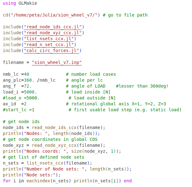
The plain Julia installation is good enough to handle the large input file and manage the large node array in a impressive fast way. I only used the fast modern plotting library GLMakie to check the imported and calculated data in 3D. So I can plot all nodes, the used load node sets and the calculated force arrows.
I still using force distribution over 72 degree to simulate a dynamic radial fatigue test according ISO 3006 (Europe) or SAE J328 (US). In this test, a constant radial force Fr is applied (see wheel with moving load for more information). Julia creates a modified input file with in that case 40 load steps. And that file can be calculated everywhere with the normal CalculiX program ccx. Afterwards we can open the calculated cxx results (*.frd) in PrePoMax to use the post processing functionalities.

I still found no way to rotate the model around the Y axis with precise angle values in PrePoMax. So I need for a rolling animation the help of the CalculiX graphical interface (CalculiX GraphiX: cgx). But the color is slightly different because there is not the same rainbow colormap available.

The implementation of the nonuniform distributed loading in Julia works much better than expected and is already better than the Ansys version implemented in APDL (wheel with moving load in Ansys). Maybe i will also add a Ansys interface to the implementation in Julia.
Julia works so fast with large files and data arrays so that you can develop new functions without any pain. Reading the input file, calculating the forces and adding the 40 steps to the input file needs only around 14 seconds and that already with a graphical output and without any optimization. Just for comparison, loading the input file (16 Mb) in a text editor (xed) already takes about 10 seconds.